Basics of Image Formation

Digital images

A raster image consists of a grid of pixels as shown in Fig. 3.

Fig. 3 An image is made from pixels. Image source wikipedia

To represent an image, we use a three dimensional array with shape (H,W,3). We say that the array has H rows, W columns and 3 color channels (red, green, and blue). Let’s load an image with python and have a look!

import numpy as np
import matplotlib.pyplot as plt
from pathlib import Path
import cv2

img_fn = str(Path("images/carla_scene.png"))
img = cv2.imread(img_fn)
# opencv (cv2) stores colors in the order blue, green, red, but we want red, green, blue
img = cv2.cvtColor(img, cv2.COLOR_BGR2RGB)

plt.imshow(img)
plt.xlabel("$u$") # horizontal pixel coordinate
plt.ylabel("$v$") # vertical pixel coordinate

print("(H,W,3)=",img.shape)

(H,W,3)= (512, 1024, 3)

Let’s inspect the pixel in the 100th row and the 750th column:

u,v = 750, 100
img[v,u]

array([28, 59, 28], dtype=uint8)

This means that the pixel at u,v = 750, 100 has a red-intensity 28, green-intensity 59, and blue-intensity 28. Hence, it is greenish. If we have a look at the image, this makes sense, since there is a tree at u,v = 750, 100. Additionally, the above output “dtype=uint8” tells us that the red, green, and blue intensities are stored as 8 bit unsigned integers, i.e., uint8. Hence, they are integers between 0 and 255.

The following sketch summarizes what we have learned about storing digital raster images so far:

Fig. 4 Image as an array of pixels.

If your digital image was taken by a camera, then there is a direct correspondence between the pixels in the digital image and “sensor pixels” in the image sensor of the camera.

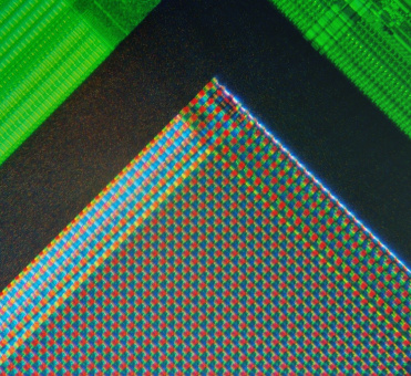
Fig. 5 Corner of the photosensor array of a webcam digital camera. Image source: wikipedia

An image sensor consists of a two dimensional array of photosensors. Each photosensor converts incoming light to electricity via the photoelectric effect, which is converted into a digital signal by means of an analog-to-digital converter. To obtain color information, one “sensor pixel” is divided into a 2 by 2 grid of photosensors, and different color filters are placed in front of these 4 photosensors. One photosensor only receives light through a blue filter, one only through a red filter, and two receive light through a green filter. Combining these 4 measurements gives one color triple: (red_intensity, green_intensity, blue_intensity). This is known as the Bayer Filter.

Fig. 6 The Bayer arrangement of color filters on the pixel array of an image sensor. Image source: wikipedia

Tip

For more details about image sensors, I recommend this youtube video.

Pinhole Camera Model

Imagine putting an image sensor in front of an object.

Fig. 7 Bad idea: Image sensor placed in front of a tree. Sketched in side view.

You would not be able to capture a sharp image like this, since a point on the image sensor will get hit by light rays from the whole environment. Now imagine putting the image sensor inside a box with a very tiny pinhole (also known as aperture).

Fig. 8 Pinhole camera.

Most of the rays are blocked now and we get a proper image on the image sensor. The image is flipped upside down, but that should not bother us. In case of an ideal pinhole, each point on the image sensor is only hit by one ray of light from the outside.

Ideal pinhole: A good approximation

In the real world the size of the hole cannot be too small because not enough light would enter the box. Additionally we would suffer from diffraction. The hole can’t be too large either, since light rays from different angles will hit the same spot on the image sensor and the image will get blurry. To act against blur, a lens is installed in real cameras. The pinhole camera model we will discuss in this section does not include the effects of a lens. However, it turns out that it is a very good approximation to cameras with lenses, and the de facto model for cameras. Hence, in the following we can continue to think of our pinhole as an ideal pinhole.

The following sketch introduces the image plane:

Fig. 9 Image formation.

While the image sensor is a distance \(f\) behind the pinhole, the so called image plane, which is an imaginary construction, is a distance \(f\) in front of the pinhole. We can relate the size \(h\) of an object to its size on the image sensor \(h'\) via similar triangles

(1)\[ \frac{h'}{h} = \frac{f}{d} \]

This means that the object size \(h'\) in the image gets smaller as the distance to the camera \(d\) increases: Far away objects appear small in an image. We can generalize Eq. (1), if we define coordinates \(x,y\) in the image plane as shown in the sketch below.

Fig. 10 Camera projection. Sketch adapted from stackexchange.

The origin of the camera coordinate system \((X_c,Y_c,Z_c)\) is at the location of the pinhole. The gray shaded region is the part of the image plane that gets captured on the image sensor. The coordinates \((u,v)\) are the pixel coordinates that were already introduced in Fig. 4. The sketch allows us to determine the mapping of a three-dimensional point \(P=(X_c, Y_c, Z_c)\) in the camera reference frame to a two-dimensional point \(p=(x,y)\) in the image plane. We have a look at the above figure in the \(Z_c\)-\(X_c\) plane:

Fig. 11 Mapping of the three-dimensional point \(P\) to the image point \(p\).

Similar triangles in the above figure reveal

\[\frac{x}{f} = \frac{X_c}{Z_c} ~ \Rightarrow ~ x = f \frac{X_c}{Z_c} \]

And similarly we find

\[ y = f \frac{Y_c}{Z_c} \]

Now, we want to establish what pixel coordinates \((u,v)\) correspond to these values of \((x,y)\) (cf. Fig. 10). First, we note that the so called principal point \((x=0,y=0)\) has the pixel coordinates \((u_0, v_0)=(W/2,H/2)\). Since \(x\) and \(y\) are measured in meters, we need to know the width and height of one “sensor pixel” in the image plane measured in meters. If the pixel width in meters is \(k_u\) and the pixel height is \(k_v\), then

(2)\[\begin{split} \begin{gather} u &= u_0 + \frac{1}{k_u}x &=u_0 + \frac{f}{k_u}\frac{X_c}{Z_c} \\ v &= v_0 + \frac{1}{k_v}y &=v_0 + \frac{f}{k_v}\frac{Y_c}{Z_c}\end{gather} \end{split}\]

If we define \(\alpha_u = f/k_u\) and \(\alpha_v = f/k_v\) we can formulate the above equations in matrix form

\[\begin{split} \begin{pmatrix} u \\ v \\ 1 \end{pmatrix} = \frac{1}{Z_c} \begin{pmatrix} \alpha_u & 0 & u_0 \\ 0 & \alpha_v & v_0 \\ 0 & 0 & 1\end{pmatrix} \begin{pmatrix} X_c \\ Y_c \\ Z_c \end{pmatrix} \end{split}\]

Typically \(\alpha_u = \alpha_v = \alpha\). To continue our discussion, we need to introduce the concept of homogeneous coordinates

Homogeneous Coordinates

We give a short informal introduction to homogeneous coordinates here. For a more detailed discussion see the book by Hartley and Zisserman ([HZ03]), or the short and long videos by Stachniss. We can convert a Euclidean vector \((u,v)^T\) into a homogeneous vector by appending a \(1\) to obtain \((u,v,1)^T\). If we multiply a homogeneous vector by a nonzero real number \(\lambda\), it is considered to still represent the same mathematical object. In other words \((u,v,1)^T\) and \(\lambda (u,v,1)^T\) are the “same” homogeneous vector, they are equivalent. Similarly \((2,3,7)^T\) and \((4,6,14)\) are equivalent. To express that two homogeneous vectors \(\mathbf{v}\) and \(\mathbf{w}\) are equivalent we write \(\lambda \mathbf{v} = \mathbf{w}\), often without exactly specifying what value \(\lambda\) has. Typically, we want to represent a homogeneous vector in its canonical form, for which the last entry is \(1\). The canonical form of \((2,3,7)^T\) is \((2/7, 3/7, 1)^T\). To go from a homogeneous vector back to a Euclidean vector, we first bringt it to canonical form, and then take all but the last vector components. In our example this would be \((2/7,3/7)^T\). Note that we can do the same procedure to construct a homogeneous vector with four components by appending a \(1\) to a three dimensional Euclidean vector. You might think that this procedure is quite strange, but soon you will see the usefulness of homogeneous coordinates.

So if we interpret the above equation as an equation for a homogeneous vector, we can absorb the scalar factor \(1/Z_c\) and rewrite the equation as

(3)\[\begin{split} \lambda \begin{pmatrix} u \\ v \\ 1 \end{pmatrix} = \begin{pmatrix} \alpha_u & 0 & u_0 \\ 0 & \alpha_v & v_0 \\ 0 & 0 & 1\end{pmatrix} \begin{pmatrix} X_c \\ Y_c \\ Z_c \end{pmatrix} \end{split}\]

If we multiply this equation by a scalar factor \(s \neq 0\), we can absorb it into \(\lambda\) on the left hand side and multiply it into the vector \((X_c,Y_c,Z_c)^T\) on the right hand side. What we find is that any point with coordinates \(s (X_c,Y_c,Z_c)^T\) will be mapped to the same \((u,v)\) coordinates. Note that all these points define a line \(\mathbf{l}(s) = s (X_c,Y_c,Z_c)^T\) which goes through the pinhole at position \((0,0,0)\). You can also verify this fact with the previous form of our equations: Eq. (2). But even more importantly, this fact is intuitive if we look at Fig. 10: Each point on the red ray from the camera origin to the point \(P\) will be mapped into the same image coordinate \((u,v)\).

Reference frames

In our applications, we will deal with with different coordinate systems, so we will not always have our point \(P\) given in coordinates of the camera reference frame \((X_c,Y_c,Z_c)^T\). For our lane-detection system the following reference frames are relevant

• World frame \((X_w, Y_w, Z_w)^T\)

• Camera frame \((X_c, Y_c, Z_c)^T\),

• Default camera frame \((X_d, Y_d, Z_d)^T\)

• Road frame \((X_r, Y_r, Z_r)^T\)

• Road frame according to ISO8855 norm \((X_i, Y_i, Z_i)^T\)

These frames are defined in the following figure

Fig. 12 Different coordinate systems. Due to the side view, only two of the three coordinate axes are drawn for most of the coordinate systems. The direction of the third coordinate axis can be inferred using the fact that all these coordinate systems are right-handed. Apart from the world frame, all frames are attached to the vehicle, which means that their origin moves with the vehicle, and their axes are defined based on the vehicle’s forwards, left, and up directions. Note that in general the \(X_w\)-\(Y_w\) plane is not parallel to the road. However, in the Carla simulator this is often the case.

The axes of the default camera frame correspond to the “right”, “down”, and “forwards” directions of the vehicle. Even if we wanted to mount our camera in a way that the camera frame equals the default camera frame, we might make some small errors. In the exercises the camera frame is slightly rotated with respect to the default camera frame, but only along the \(X_d\)-axis: The camera has a pitch angle of 5°.

In the following we will describe how to transform between world and camera coordinates, but the same mathematics hold for a transformation between any two of the the above reference frames. A point \((X_w, Y_w, Z_w)^T\) in the world coordinate system is mapped to a point in the camera coordinate system via a rotation matrix \(\bf{R} \in \mathbb{R}^{3 \times 3}\) (to be more precise \(\mathbf{R} \in SO(3)\)) and a translation vector \(\bf{t}\)

\[\begin{split} \begin{pmatrix} X_c \\ Y_c \\ Z_c \end{pmatrix} = \bf{R} \begin{pmatrix} X_w \\ Y_w \\ Z_w \end{pmatrix} + \bf{t} \end{split}\]

We can write this transformation law just using matrix multiplication

(4)\[\begin{split} \begin{pmatrix} X_c \\ Y_c \\ Z_c \\ 1 \end{pmatrix} =\begin{pmatrix} R_{xx} & R_{xy} & R_{xz} & t_x \\ R_{yx} & R_{yy} & R_{yz} & t_y \\ R_{zx} & R_{zy} & R_{zz} & t_z \\ 0 & 0 & 0 & 1 \end{pmatrix} \begin{pmatrix} X_w \\ Y_w \\ Z_w \\ 1\end{pmatrix} = \mathbf{T}_{cw} \begin{pmatrix} X_w \\ Y_w \\ Z_w \\ 1\end{pmatrix} \end{split}\]

where we defined the transformation matrix \(\bf{T}_{cw}\) in the last equality. It is great that we can relate the coordinates of different reference frames just by using a matrix. This makes it easy to compose several transformations, for example to go from world to camera coordinates and then from camera to road coordinates. It also enables us to get the inverse transformation using the matrix inverse: The transformation from camera to world coordinates is given by the matrix \(\bf{T}_{wc} = \bf{T}_{cw}^{-1}\).

To conclude this section, we combine Eq. (3) and (4) into one single equation:

(5)\[\begin{split} \lambda \begin{pmatrix} u \\ v \\ 1 \end{pmatrix} = \begin{pmatrix} \alpha_u & 0 & u_0 \\ 0 & \alpha_v & v_0 \\ 0 & 0 & 1\end{pmatrix} \begin{pmatrix} R_{xx} & R_{xy} & R_{xz} & t_x \\ R_{yx} & R_{yy} & R_{yz} & t_y \\ R_{zx} & R_{zy} & R_{zz} & t_z \end{pmatrix} \begin{pmatrix} X_w \\ Y_w \\ Z_w \\ 1\end{pmatrix} \end{split}\]

Or by defining the intrinsic camera matrix \(\mathbf{K}\) and the extrinsic camera matrix \(\begin{pmatrix} \mathbf{R} | \mathbf{t} \end{pmatrix}\)

(6)\[\begin{split} \lambda \begin{pmatrix} u \\ v \\ 1 \end{pmatrix} = \mathbf{K} \begin{pmatrix} \mathbf{R} | \mathbf{t} \end{pmatrix} \begin{pmatrix} X_w \\ Y_w \\ Z_w \\ 1\end{pmatrix} \end{split}\]

Yaw, pitch, and roll rotations

Before you start the exercises, you should briefly be introduced to the yaw, pitch, and roll parametrization of rotations: A general rotation between the camera frame and the default camera frame can be described by first rotating for some angle (called roll angle) around the \(Z_d\)-axis, then for some other angle (called pitch angle) around the \(X_d\)-axis, and finally for even another angle (called yaw angle) around the \(Y_d\)-axis.

If we define the cosine and sine of the roll angle as \(c_r\) and \(s_r\) respectively, the roll rotation matrix is

\[\begin{split}R_{roll} = \begin{pmatrix}c_{r} & - s_{r} & 0\\s_{r} & c_{r} & 0\\0 & 0 & 1\end{pmatrix}\end{split}\]

Defining cosine and sine of the pitch angle as \(c_p\) and \(s_p\) and the cosine and sine of the yaw angle as \(c_y\) and \(s_y\), the pitch and yaw rotation matrices are

\[\begin{split}R_{pitch} = \begin{pmatrix}1 & 0 & 0\\0 & c_{p} & s_{p}\\0 & - s_{p} & c_{p}\end{pmatrix}\end{split}\]

\[\begin{split}R_{yaw} = \begin{pmatrix}c_{y} & 0 & - s_{y}\\0 & 1 & 0\\s_{y} & 0 & c_{y}\end{pmatrix}\end{split}\]

Note that the form of these matrices depends on the coordinate system. We chose the \((X_d, Y_d, Z_d)^T\) frame here. In the \((X_i, Y_i, Z_i)^T\) frame the matrices would look a bit different, since for example the “forwards” direction in the \((X_i, Y_i, Z_i)^T\) frame is \((1,0,0)^T\), whereas it is \((0,0,1)^T\) in the default camera frame \((X_d, Y_d, Z_d)^T\). So if you find a differently looking roll matrix in some book, this probably has to do with the naming of the axes. What all books tend to agree on: In the case of vehicles (like cars or planes), the roll axis points forwards, the yaw axis upwards (or downwards), and the pitch axis to the right (or left).

Fig. 13 Yaw, pitch, and roll rotations. The orange arrow on the pitch axis indicates that “lifting up its nose” will increase the pitch angle of the airplane. So it indicates the sign convention for the angle. Not all text books agree on common sign conventions here. wikipedia

A general rotation can be written by multiplying the roll, pitch, and yaw matrices

(7)\[\begin{split} R = R_{yaw} R_{pitch} R_{roll} = \begin{pmatrix}c_{r} c_{y} + s_{p} s_{r} s_{y} & c_{r} s_{p} s_{y} - c_{y} s_{r} & - c_{p} s_{y}\\c_{p} s_{r} & c_{p} c_{r} & s_{p}\\c_{r} s_{y} - c_{y} s_{p} s_{r} & - c_{r} c_{y} s_{p} - s_{r} s_{y} & c_{p} c_{y}\end{pmatrix} \end{split}\]

In the exercise code, we will parametrize the rotation matrix that rotates vectors from the road frame into the camera frame using the formula above. Note that the axis directions of the road frame and the default camera frame are identical.

For the purpose of this chapter, we will be happy with parametrizing a rotation matrix via yaw, pitch, and roll. However there are some problems with this representation. Three dimensional rotations are more complicated than you might think. If you want to learn more I recommend this YouTube video by Cyrill Stachniss.

Exercise: Projecting lane boundaries into an image

Now you should start to work on your first exercise. For this exercise, I have prepared some data for you. I captured an image in the Carla simulator using a camera sensor attached to a vehicle:

Fig. 14 Image captured by a camera sensor in a Carla simulation.

Additionally I created txt files containing

• world coordinates of the lane boundaries \((X_w,Y_w,Z_w)^T\)

• a transformation matrix \(T_{cw}\) that maps world coordinates to coordinates in the camera reference frame

Your job is to write code based on equation (6) that creates a label image like this:

Fig. 15 Label image.

First you will need to set up your python environment, install the necessary libraries, and download the code for the exercises. Please visit the appendix to learn how.

To start working on the exercises, open code/tests/lane_detection/lane_boundary_projection.ipynb and follow the instructions in that notebook.

References

HZ03

Richard Hartley and Andrew Zisserman. Multiple view geometry in computer vision. Cambridge university press, 2003.