From Pixels to Meters

Inverse perspective mapping

Having detected which pixel coordinates \((u,v)\) are part of a lane boundary, we now want to know which 3 dimensional points \((X_c,Y_c,Z_c)^T\) correspond to these pixel coordinates \((u,v)\). First let us have a look at this sketch of the image formation process again:

Fig. 16 Camera projection. Sketch adapted from stackexchange.

Remember: Given a 3 dimensional point in the camera reference frame \((X_c,Y_c,Z_c)^T\), we can obtain the pixel coordinates \((u,v)\) via

\[\begin{split} \lambda \begin{pmatrix} u \\ v \\ 1 \end{pmatrix} = \mathbf{K} \begin{pmatrix} X_c \\ Y_c \\ Z_c \end{pmatrix} \end{split}\]

But what we need to do now is solve the inverse problem. We have \((u,v)\) given, and need to find \((X_c,Y_c,Z_c)^T\). To do that, we multiply the above equation with \(\mathbf{K}^{-1}\):

\[\begin{split} \begin{pmatrix} X_c \\ Y_c \\ Z_c \end{pmatrix} = \lambda \mathbf{K}^{-1} \begin{pmatrix} u \\ v \\ 1 \end{pmatrix} \end{split}\]

Our problem is that we do not know the value of \(\lambda\). This means that the 3d point \((X_c,Y_c,Z_c)^T\) corresponding to pixel coordinates \((u,v)\) is somewhere on the line defined by

\[\begin{split} \mathbf{r}(\lambda) = \lambda \mathbf{K}^{-1} \begin{pmatrix} u \\ v \\ 1 \end{pmatrix}, ~ \lambda \in \mathbb{R}_{>0} \end{split}\]

But which \(\lambda\) yields the point that was captured in our image? In general, this question cannot be answered. But here, we can exploit our knowledge that \(\mathbf{r}(\lambda)\) should lie on the road! It corresponds to a point on the lane boundary after all. We will assume that the road is planar. A plane can be characterized by a normal vector \(\mathbf{n}\) and some point lying on the plane \(\mathbf{r}_0\):

\[ \textrm{Point } \mathbf{r} \textrm{ lies in the plane} ~ \Leftrightarrow ~ \mathbf{n}^T (\mathbf{r} - \mathbf{r}_0) = 0 \]

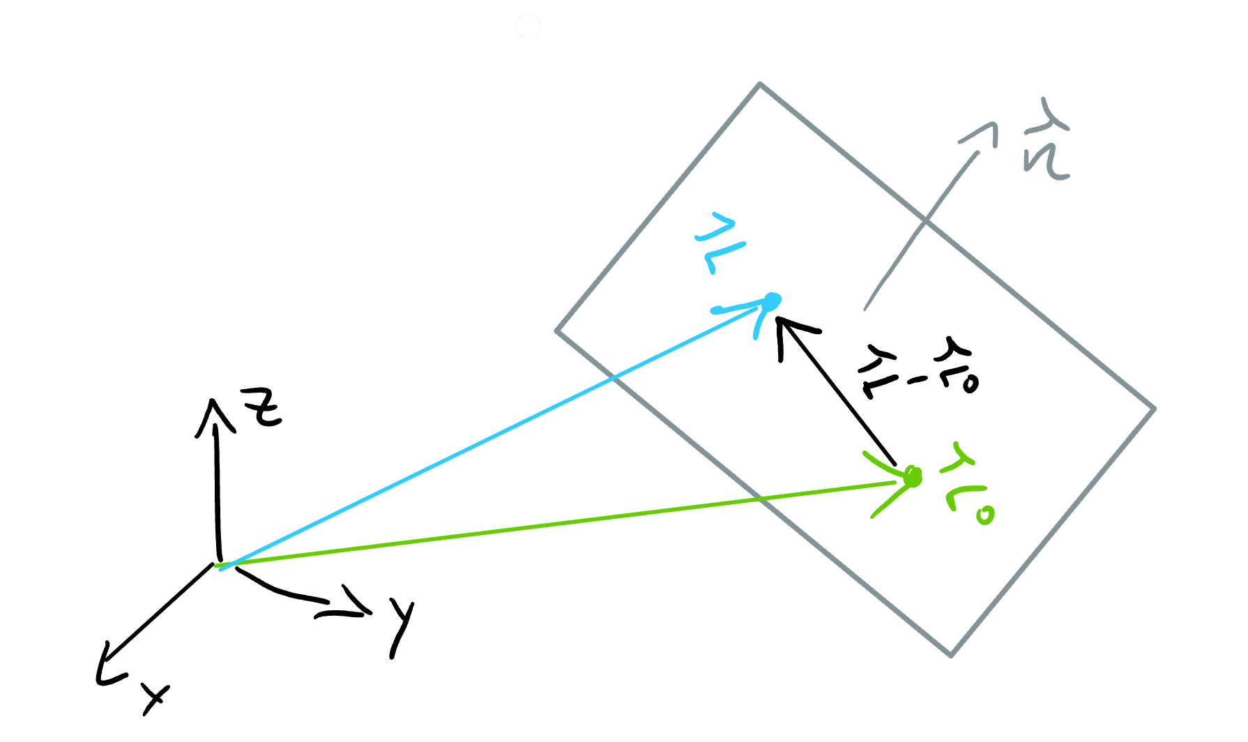
Fig. 17 Equation for a planar surface

In the road reference frame the normal vector is just \(\mathbf{n} = (0,1,0)^T\). Since the optical axis of the camera is not parallel to the road, the normal vector in the camera reference frame is \(\mathbf{n_c} = \mathbf{R_{cr}} (0,1,0)^T\), where the rotation matrix \(\mathbf{R_{cr}}\) describes how the camera is oriented with respect to the road: It rotates vectors from the road frame into the camera frame. The remaining missing piece is some point \(\mathbf{r}_0\) on the plane. In the camera reference frame, the camera is at position \((0,0,0)^T\). If we denote the height of the camera above the road by \(h\), then we can construct a point on the road by moving from \((0,0,0)^T\) in the direction of the road normal vector \(\mathbf{n_c}\) by a distance of \(h\): Hence, we pick \(\mathbf{r}_0 = h \mathbf{n_c}\), and our equation for the plane becomes \(0= \mathbf{n_c}^T (\mathbf{r} - \mathbf{r}_0) = \mathbf{n_c} ^T \mathbf{r} - h\) or \(h=\mathbf{n_c}^T\mathbf{r}\).

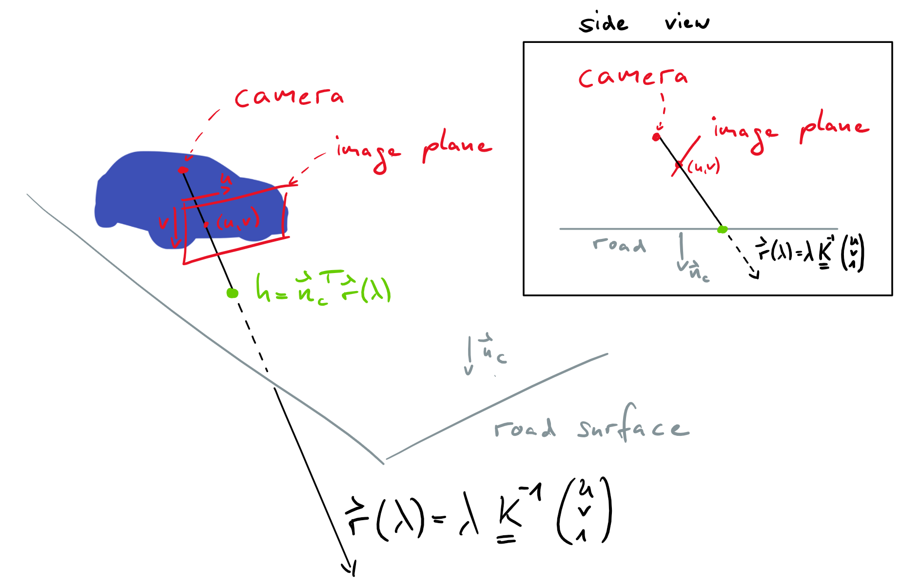
Fig. 18 Finding the correct \(\lambda\)

Now we can compute the point where the line \(\mathbf{r}(\lambda) = \lambda \mathbf{K}^{-1} (u,v,1)^T\) hits the road, by plugging \(\mathbf{r}(\lambda)\) into the equation of the plane \(h=\mathbf{n_c}^T\mathbf{r}\)

\[ h = \mathbf{n_c}^T \lambda \mathbf{K}^{-1} (u,v,1)^T ~ \Leftrightarrow~ \lambda = \frac{h}{ \mathbf{n_c}^T \mathbf{K}^{-1} (u,v,1)^T} \]

We can now plug this value of \(\lambda\) into \(\mathbf{r}(\lambda)\) to obtain the desired mapping from pixel coordinates \((u,v)\) to 3 dimensional coordinates in the camera reference frame

(8)\[\begin{split} \begin{pmatrix} X_c \\ Y_c \\Z_c \end{pmatrix} = \frac{h}{ \mathbf{n_c}^T \mathbf{K}^{-1} (u,v,1)^T} \mathbf{K}^{-1} \begin{pmatrix} u \\ v \\ 1 \end{pmatrix} \end{split}\]

This equation is only true if the image shows the road at pixel coordinates \((u,v)\). It may look a bit ugly, but it is actually pretty easy to implement with python.

Exercise: Inverse perspective mapping

In this exercise you will implement Eq. (8) as well as the coordinate transformation between the camera reference frame and the road reference frame. For the latter part, you might look back into Basics of Image Formation. Note that you should have successfully completed the exercise in Basics of Image Formation before doing this exercise.

To start working on the exercise, open code/tests/lane_detection/inverse_perspective_mapping.ipynb and follow the instructions in that notebook.

Fitting the polynomial

Our aim is to obtain polynomials \(y_l(x)\) and \(y_r(x)\) describing the left and right lane boundaries in the road reference frame (based on ISO 8855).

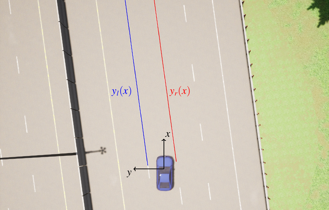
Fig. 19 Our aim is to find \(y_l(x)\) and \(y_r(x)\)

import numpy as np
import matplotlib.pyplot as plt

From Lane Boundary Segmentation we know that our semantic segmentation model will take the camera image as input and will return a tensor output of shape (H,W,3). In particular prob_left = output[v,u,1] will be the probability that the pixel \((u,v)\) is part of the left lane boundary. I saved the tensor output[v,u,1] that my neural net computed for some example image in a npy file. Let’s have a look

prob_left = np.load("../../data/prob_left.npy")
plt.imshow(prob_left, cmap="gray")
plt.xlabel("$u$");
plt.ylabel("$v$");

The image above shows prob_left[v,u] for each (u,v). Now imagine that instead of triples (u,v,prob_left[v,u]) we would have triples (x,y,prob_left(x,y)), where \((x,y)\) are coordinates on the road like in Fig. 19. If we had these triples we could filter them for all (x,y,prob_left[x,y]) where prob_left[x,y] is large. We would obtain a list of points \((x_i,y_i)\) which are part of the left lane boundary and we could use these points to fit our polynomial \(y_l(x)\)! But going from (u,v,prob_left[v,u]) to (x,y,prob_left[x,y]) is actually not that hard, since you implemented the function uv_to_roadXYZ_roadframe_iso8855 in the last exercise. This function converts \((u,v)\) into \((x,y,z)\) (note that \(z=0\) for road pixels).

That means we can start and write some code to collect the triples (x,y,prob_left[x,y])

import sys
sys.path.append('../../code')
from solutions.lane_detection.camera_geometry import CameraGeometry
cg = CameraGeometry()

xyp = []
for v in range(cg.image_height):
    for u in range(cg.image_width):
        X,Y,Z= cg.uv_to_roadXYZ_roadframe_iso8855(u,v)
        xyp.append(np.array([X,Y,prob_left[v,u]]))
xyp = np.array(xyp)

I mention flatten here because it is well known. But in our case, it is actually better to use np.ravel().

This double for loop is quite slow, but don’t worry. The first two columns of the xyp array are independent of prob_left, and hence can be precomputed. The last column can be computed without a for loop: xyp[:,2]==prob_left.flatten(). You will work on the precomputation in the exercise.

To restrict ourselves to triples (x,y,prob_left[x,y]) with large prob_left[x,y] we can create a mask. Then, we can insert the masked x and y values into the numpy.polyfit() function, to finally obtain our desired polynomial \(y(x)=c_0+c_1 x+ c_2 x^2 +c_3 x^3\). The numpy.polyfit() performs a least squares fit. But it can even do a weighted least squares fit if we pass an array of weights. We will just pass the probability values as weights, since (x,y) points with high probability should be weighted more.

x_arr, y_arr, p_arr = xyp[:,0], xyp[:,1], xyp[:,2]
mask = p_arr > 0.3
coeffs = np.polyfit(x_arr[mask], y_arr[mask], deg=3, w=p_arr[mask])
polynomial = np.poly1d(coeffs)

Let’s plot our polynomial:

x = np.arange(0,60,0.1)
y = polynomial(x)
plt.plot(x,y)
plt.xlabel("x (m)"); plt.ylabel("y (m)"); plt.axis("equal");

Looks good!

Encapsulate the pipeline into a class

You have seen both steps of our lane detection pipeline now: The lane boundary segmentation, and the polynomial fitting. For future usage, it is convenient to encapsulate the whole pipeline into one class. In the following exercise, you will implement such a LaneDetector class. For now, let’s have a look at the sample solution for the LaneDetector in action. First, we load an image

import cv2

img_fn = "images/carla_scene.png"
img = cv2.imread(img_fn)
img = cv2.cvtColor(img, cv2.COLOR_BGR2RGB)
plt.imshow(img);

Now we import the LaneDetector class and create an instance of it. For that we specfiy the path to a model that we have stored with pytorch’s save function.

from solutions.lane_detection.lane_detector import LaneDetector
model_path ="../../code/solutions/lane_detection/fastai_model.pth"
ld = LaneDetector(model_path=model_path)

From now on we can get the lane boundary polynomial for any image (that is not too different from the training set) by passing it to the ld instance.

poly_left, poly_right = ld(img)

On Google Colab this call takes around 45 ms. This is not quite good enough for real time applications, where you would expect 10-30 ms or less, but it is close. The bottleneck of this sample solution is the neural network. Maybe you implemented a more efficient one? If you want to make the system faster, you could also consider feeding lower resolution images into the network - both during training and inference. This would trade off accuracy for speed. If you try it out let me know how well it works ;)

Now let’s have a look at the polynomials that ld has computed

x = np.linspace(0,60)
yl = poly_left(x)
yr = poly_right(x)
plt.plot(x, yl, label="yl")
plt.plot(x, yr, label="yr")
plt.xlabel("x (m)"); plt.ylabel("y (m)");
plt.legend(); plt.axis("equal");

(-3.0, 63.0, -1.984601121412455, 4.112957019939879)

This looks quite reasonable. In the next exercise, you will create a similar plot and compare it to ground truth data from the simulator.

Exercise: Putting everything together

For the final exercise, you will implement polynomial fitting, and then encapsulate the whole pipeline into the LaneDetector class. To start, go to code/tests/lane_detection/lane_detector.ipynb and follow the instructions.

Tip for fastai users

If you trained your model with fastai, you could use Learner.predict() to get the model output for one image. But sadly this is super slow. You can use this python function for faster computation:

def get_prediction(model, img_array):
    with torch.no_grad():
        image_tensor = img_array.transpose(2,0,1).astype('float32')/255
        x_tensor = torch.from_numpy(image_tensor).to("cuda").unsqueeze(0)
        model_output = F.softmax(model.forward(x_tensor), dim=1 ).cpu().numpy() 
        # maybe for your model you need to replace model.forward with model.predict in the line above
    return model_output
# usage example:
model = torch.load("fastai_model.pth").to("cuda")
model.eval()
image = cv2.imread("some_image.png")
image = cv2.cvtColor(image, cv2.COLOR_BGR2RGB)
get_prediction(model, image)

If you want to know why this works, you can read this blog post, where the section “A simple example” explains what happens inside Learner.predict() under the hood.